Theory and an Idea of SSA

Singular Spectrum Analysis is a method which is the consequence of many different results in Multivariate Statistics, Linear Algebra, and its crucial embedding stage being inspired possibly by a number of different sources, but often accepted to be a result of work within Dynamical Systems. Once the embedding step is performed we have converted our 1D data into a multidimensional system which can then be analyzed by methods like PCA and Karhunen-Loe`ve transform.

While a thorough study of these theorems is much too interesting, they are not required for developing the algorithm necessarily. Our approach will be to focus on building an intuition as to why SSA works by examining the embedding stage, SVD, and a crucial concept for understanding its results, separability. The mathematical rigor is sacrificed in support of better developing the algorithm and examining its applications.

We will begin with a brief history. Then focusing on the first stage of SSA, Decomposition, which has two steps : Embedding and SVD will be discussed in depth as they are the most involved in terms of theory and why we do them, but rather minimal in their implementation. The second stage, Reconstruction has two steps : Grouping and Diagonal Averaging. Both rather easy to grasp, but a bit more involved in terms of their implementation and hence will be focused on more in that section.

A brief History

As mentioned earlier, the embedding stage is a crucial distinguishing step in SSA. SSA as a method is first said to be introduced in publication of papers by Broomhead and King (1986a, 1986b) and Broomhead et al. (1987). These papers highlighted and introduced the key stage of embedding, as a result of the Taken Theorem in Dynamical Systems. This allowed a analysis of a observed time series as if it was multivariate data.

SSA gained much traction after its use in analysis of climatic, meteorological and geophysical data, specifically by papers from Vautard and Ghil in 1989 and 1991. Around the same time a crucial resource was published on SSA by Elsner & Tsonis in 1996, titled “Singular Spectrum Analysis : A new tool in Time Series Analysis”, the book follows the same style of algorithm and approach to SSA as Vautard and Ghil. In parallel, SSA was also being developed in Russia, with the name ‘Caterpillar Method’. SSA as it is recognized today was mainly a result of the monograph, Golyandina et al. (2001). In my study of this method many of the current stylistic choices and development of the algorithm is done by the same authors in a number of papers and 2 other books. They also developed the current SSA package within R.

Embedding : Low Rank Matrices and Redundancy

The embedding stage of SSA can be understood by approaching it from a number of ways. A great mathematical justification for embedding is given in Elsner and Tsonis (1996), which shows its roots in Takens Embedding theorem.

To continue with our goal for a more intuitive approach, we will begin with examining the step directly to infer it’s advantages and justification.

The goal of Embedding is to create what will be referred to as the Trajectory Matrix,
Here we take our 1D data vector and create lagged copies of it. The idea roughly is this. If there is some sort of seasonality or trend within our data, it must persist through the time series. Instead of looking at the time series as a whole we choose a set length, we will call $L$, and then find structure within subsets of the original data of length, $L$, that are shifted.

We can visualize this by creating heatmaps of a 1D vector and then creating its trajectory matrix.

Let us observe a toy signal

$$x = [1, 0, -1, 0, 1, 0, -1, 0, 1, 0]$$

The choice of our parameter $L$ is discussed later in this paper, for now let us set $L = 4$. Now, Given our total length of the vector being $N=10$, we have $K=N-L+1$ lagged vectos, which is $K = 10 - 4 + 1 = 7$, which are

$$\begin{aligned} x_1 &= [1, 0, -1, 0] \\ x_2 &= [0, -1, 0, 1] \\ x_3 &= [-1, 0, 1, 0] \\ x_4 &= [0, 1, 0, -1] \\ x_5 &= [1, 0, -1, 0] \\ x_6 &= [0, -1, 0, 1] \\ x_7 &= [-1, 0, 1, 0] \end{aligned}$$

we can then stack them into a matrix,

$$X = \begin{bmatrix} x_1 \\ x_2 \\ x_3 \\ x_4 \\ x_5 \\ x_6 \\ x_7 \end{bmatrix} = \begin{bmatrix} 1 & 0 & -1 & 0 \\ 0 & -1 & 0 & 1 \\ -1 & 0 & 1 & 0 \\ 0 & 1 & 0 & -1 \\ 1 & 0 & -1 & 0 \\ 0 & -1 & 0 & 1 \\ -1 & 0 & 1 & 0 \end{bmatrix}$$

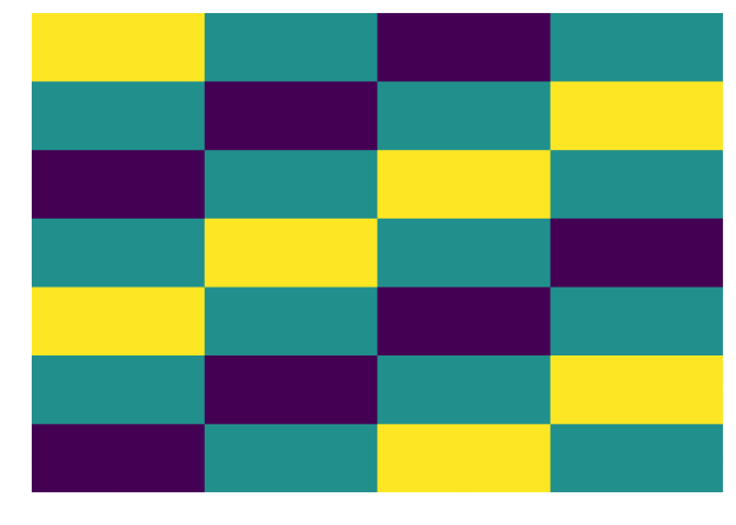
When we analyze the trajectory matrix, we come up with two important observations : that it is Rank deficient, and a Hankel Matrix. The second is simply a structural observation we can verify by looking at all the anti-diagonals and confirming that each is made of a single value, or in our heatmap, color.

This observation allows us to also use the formula for a Hankel Matrix to code our first step in our SSA implementation as well. Given a parameter $L$, and the length of our observed signal, $N$ and $K$, we get a $K \times L$ trajectory matrix X, which is defined as :

$$X_{i,j} = x_{i+j-1} \qquad(1)$$

We will refer to this operation by defining it as a operator, the embedding operator, $\mathcal{H}$. It is also obvious that it is a linear operator as it only rearranges the series into a matrix.

$$\mathcal{H}(x)= \begin{pmatrix} x_1 & x_2 & \cdots & x_L \\ x_2 & x_3 & \cdots & x_{L+1} \\ \vdots & \vdots & \ddots & \vdots \\ x_K & x_{K+1} & \cdots & x_N \end{pmatrix}$$

The observation that it is Rank Deficient is obvious after we do its RREF, we find that we only need two of the columns or the row to express the rest. This is a crucial observation and a condition that when met can allow us to exract patterns or trends from our signal/time series.

Another way to think about this is that if there is any pattern or structure within our time series. The rank of the Trajectory matrix is the number of independent patterns that describe our signal. Our goal now becomes to extract these components. This is done by taking the SVD of our trajectory matrix

Singular Value Decomposition

This is a Decomposition method which can find unique decomposition of any rectangular matrix, by finding its singular vectors and singular directions.

Given a matrix $A$ which is $n\times m$

$$A = U\Sigma V^\top$$

Where $U$ is matrix of the form $[u_1, u_2, ... , u_r]$ where each column is made up of $u$, called the left singular vectors, and V is matrix of the form $[v_1,v_2,...,v_r]$ where each column is made up of $v$, called the right singular vectors. Here $r$, is the rank of the trajectory matrix.

$\Sigma$ is a diagonal matrix for which the non-zero values are called the singular values.

A derivation of the decomposition, can be simply done by assuming such a decomposition exists, and then taking the spectral decomposition of the $AA^\top$ and $A^\top A$ matrix.

Assuming, $A = U\Sigma V^\top$ and as both $AA^\top$ and $A^\top A$ are symmetric, so have a spectral decomposition.

$$\begin{aligned} AA^\top = PDP^\top = (U\Sigma V^\top)(U\Sigma V^\top)^\top\\ PDP^\top = (U\Sigma V^\top)(V \Sigma^\top U^\top) \\ PDP^\top = (U\Sigma^2 U^\top) \\ P = U, D = \Sigma^2 \\ \end{aligned}$$ $$\begin{aligned} A^\top A = PDP^\top = (U\Sigma V^\top)^\top(U\Sigma V^\top) \\ PDP^\top = (V \Sigma^\top U^\top)(U\Sigma V^\top) \\ PDP^\top = (V \Sigma^2 V^\top) \\ P = V, D = \Sigma^2 \end{aligned}$$

This gives

• $U$ is made up of the eigenvectors of the $AA^\top$ matrix. It is a orthogonal matrix
• $V$ is made up of the eigenvectors of the $A^\top A$ matrix. It is also a orthogonal matrix
• The singular values are the square roots of the non-zero eigenvalues of either matrix as they are the same. These values are often notated as $\sigma_i$. They are ordered as $\sigma_1 \geq \sigma_2 \geq ... \geq \sigma_i$. The corresponding singular values are ordered accordingly in $U$ and $V$.

This decomposition also allows us to re-express our matrix as a sum of rank-1 biorthogonal matrices.

$$A = \sum_{i=1}^{r} \sigma_i u_i v_i^\top$$

Each rank-1 matrix is made up of its own eigentriple ($u_iv_i\sigma_i$). These eigentriples correspond to independent structures within our trajectory matrix. Each rank-one matrix represents a pattern consisting of a fixed structure that is repeated across the trajectory matrix with varying intensity.

It is important to highlight two important optimal features of SVD here.

First, that for $k<r=rank(A)$ let the truncated SVD matrix, $A_k$ be defined as

$$A_k = \sum_{i=1}^k \sigma_i u_i v_i^\top$$

and the Frobenius norm is

$$\|A\|_F = \left( \sum_{i=1}^m \sum_{j=1}^n a_{ij}^2 \right)^{1/2} \qquad(2)$$

Equivalently, the Frobenius norm may be written using the trace as

$$\|A\|_F^2 = \operatorname{tr}(A^\top A). \qquad(3)$$

So, Under the Frobenius norm, among all matrices of rank $k<r$, $A_K$ provides the best approximation to the original matrix A.

$$\|A - A_k\|_F = \min_{\operatorname{rank}(B)\le k} \|A-B\|_F. \qquad(4)$$

Also note that

$$\|A\|_F^2 = \sum_{i=1}^r \sigma_i^2$$

now as the same follows for the truncated matrix,

$$\|A_k\|_F^2 = \sum_{i=1}^k \sigma_i^2$$

We can see that

$$\frac{\sum_{i=1}^k \sigma_i^2}{\sum_{i=1}^r \sigma_i^2}$$

This is the contribution of the truncated SVD to the whole trajectory matrix. Using this to interpret the idea of contribiton of each rank-1 matrix we have that contribution of these matrices is just the singular value associated with them. This result will allow us to develop an way of quantifying and obtaining our groups for components and the final smoothing.

The other optimality feature is a bit more involved in terms of its proof, and is also a important result that makes SVD important in Principal Component Analysis.

It is roughly relates to the properties of the directions determined by the eigenvectors $v_1,v_2,v_3,...v_r$. Specifically, the first eigenvector $v_1$ determines the direction such that the variation of the projections of the lagged vectors onto this direction is maximum. This helps us have an intuiton as to why the noise in our signal would be the one associated with the smallest eigenvalues. Noise tends to spread across many directions rather than concentrating in a single dominant direction, and therefore is associated with smaller singular values.

The next step in SSA is to determine how these elementary components can be grouped and then reconstructed to recover interpretable features such as trends and oscillations.

Grouping

This a good place for us to to review our goal with SSA. To extract components from the original time series that when summed give us the original time series. These components then can be interpreted as Trend or Periodic or quasi-periodic components.

$$S = T + P + N \qquad(5)$$

and

We also will describe the naive signal model, where the trend and periodic components add up to make our original Signal.

$$S = S_{signal} + N$$

Here, T corresponds to the trend, overall direction the signal takes, and P is the seasonal quasi-periodic component. N corresponds to the residual or noise within the observed signal.

Now, using our embedding operator on Equation 5, we have the following

$$\begin{aligned} \mathcal{H}(S) = \mathcal{H}(T) + \mathcal{H}(P) + \mathcal{H}(N) \\ = X_S = X_T + X_P + X_N \end{aligned} \qquad(6)$$

Comparing this with taking the SVD of the hankel/trajectory matrix $X_S$, we have

$$\begin{aligned} X_S = X_1 + X_2 + X_3 + ... + X_r \\ X_S = X_T + X_P + X_N \end{aligned} \qquad(7)$$

This gives us our motivation for grouping. We need to find disjoint subsets of indices from the total rank of our Trajectory matrix, where for each we can add its corresponding rank-1 matrices to calculate the Hankel versions of the specific component we are interested in, like trend or oscillation.

Although the SVD expresses the trajectory matrix as a sum of bi-orthogonal rank-one components, these do not necessarily correspond to interpretable features of the signal. In practice, meaningful structures such as trends or oscillations are often represented by multiple singular components. The purpose of grouping is therefore to combine related elementary components into larger structures that reflect the true underlying behavior of the time series.

But it is important to highlight that there is a condition which must be met for such groups to exist. The component features of the series must be seperable for us to find these groups of indices, for which the corresponding trajectory matrices can be obtained.

While due to the optimality feature of SVD, specifically one where the noise tends to be associated with small singular values allows us to split the signal in two separate groups, and accordingly two separate trajectory matrices. For extraction of feature components like Trend, Periodicty or Oscillation, this becomes a much more involved process.

We will discuss the idea of separability once we introduce the manner by which we can convert any matrix to its Hankel version and then extract a time series associated with it.

Diagonal Averaging : The Hankelization Operator

This is the last step in terms of obtaining components of the original signal or time series that we are interested in. Given some timeseries of length $N$, $x_N$. Its trajectory matrix, given a window length of $L$ is $\mathcal{H}(x_N) = X$. Taking its SVD and finding $m$ groups that we are interested in gives the following.

$$X_m1, X_m2, ... X_m$$

These are the matrices from which we want to obtain a vector which would be associated with a Trend or period or some interpretable component.

The method of Diagonal Averaging does that for us. The idea is as the values of the original signal lie on each anti-diagonal. We should be able to extract the associated signal for each component by looking at the anti-diagonals of the associated component Trajectory matrix.

For this to be the case, we need these matrices to be Hankel in nature. For which we introduce the Hankelization Operator, $\mathcal{D}$. The formal defintion of this operator is the following

$$\widetilde{y}_{ij} = \begin{cases} \dfrac{1}{s-1}\displaystyle\sum_{l=1}^{s-1} y_{l,\,s-l}, & \text{for } 2 \leq s \leq L-1, \\[1.2em] \dfrac{1}{L}\displaystyle\sum_{l=1}^{L} y_{l,\,s-l}, & \text{for } L \leq s \leq K+1, \\[1.2em] \dfrac{1}{K+L-s+1}\displaystyle\sum_{l=s-K}^{L} y_{l,\,s-l}, & \text{for } K+2 \leq s \leq K+L. \end{cases}$$

This operator when applied on the groupings gives a unique matrix for each group, consequently giving a associated time series for each group. But as it only takes a matrix and is a linear operator, we can always just apply this to every rank-1 matrix, and then add the term series to get total series for each group. This gives us our goal decomposition of the original time series.

The implementation of this operator is a bit different then the formal defintion, for which we only need to observe two facts about this. First, that the anti-diagonals have each component have their indices value equal to a constant. And that this operator simply sums the values on these anti-diagonals and divides them by the number of component in the diagonal, hence Diagonal Averaging.

Separability

Given a time series, $F$, lets say the decomposed version is $F = F^{(1)} + F^{(2)}$. The goal with SSA, specifically the grouping step becomes to identify the groupes of rank-1 matrices that produce corresponding trajectory matrices.

So we get a decomposition of our trajectory matrix, $X$, as $X = X^{(1)} + X^{(2)}$. For such groupings to exist that we can calculate $X^{(1)}$ or $X^{(2)}$ such that we can recover $F^{(1)}$ and $F^{(2)}$, the two components need to be seperable.

The idea can roughly be understood as, two components are separable if their contributions to the trajectory matrix are sufficiently distinct that the SVD can assign them to different eigentriples or different groups of eigentriples.

We have two notions of separability, Weak and Strong separability. We will mainly focus on Weak separability as it allows us to build a more clear way of implimenting SSA.

Weak separability

Here, two components, $F^{(1)}$ and $F^{(2)}$, are weakly seperable when their corresponding trajectory matrices, $X^{(1)}$ or $X^{(2)}$ are orthogonal. So the column space and the row space of the two matrices are orthogonal to each other.

A standard way to calculate this is the Frobenius Orthogonality.

$$\langle X^{(1)}, X^{(2)} \rangle_F = 0.$$ $$\langle A, B \rangle_F = \sum_{i=1}^{K}\sum_{j=1}^{L} a_{ij}b_{ij}.$$

Now as we discussed in the previous section. The reconstructed series from their corresponding matrices are actually extracted from an Hankelized version of that matrix. So instead there is another operator developed which measures the weak separability between reconstructed series.

This is called the W-orthogonality condition. When two series are seperable, their W-orthogonality is exactly 0.

We usually also calculate a w-correlation matrix, which helps us understand how close we are to this separability measure. We can simply understand this as the cosine of the angle between the space formed by the trajectory matrices.

It can be calculated in the following manner :

Given the weighted inner product as

$$\langle F^{(1)}, F^{(2)} \rangle_w = \sum_{i=1}^{N} w_i \, x_i y_i$$

Here the weight is the number of times each term of the series shows up on the diagonal of its associated Hankel Matrix.

Now when $\langle F^{(1)}, F^{(2)} \rangle_w = 0$ it implies a orthogonality of the trajectory matrix.

The W-correlation matrix then is defined as

$$\rho^w_{(i,j)} = \frac{\langle F^{(1)}, F^{(2)} \rangle_w}{\|F^{(1)}\|_w \|F^{(2)}\|_w}$$

where, $\|F^{(i)}\|_w = \sqrt{\langle F^{(1)}, F^{(1)} \rangle_w}$

So for values of this matrix range between -1 to 1. But in practice we usually consider the absolute value of the matrix. All the diagonal values are 1, as two series are exactly related to themselves. All values close to 1, can be grouped together and those with close to 0 are seperable.

Strong separability

The notion of strong separability is simply extending weak separability with the condition that the singular values of any two groups are disjoint.

This confirms unique SVD rank-1 matrices ensuring a clean seperation.

Implementation

Now we will focus on implimenting a Basic SSA algorithm

A note on style and focus on efficiency

This version of the algorithm is heavily inspired by the work of N. Golyandina. specifically the algorithm and its theory as described in Golyandina and Zhigljavsky (2020), and Golyandina et al. (2001).

The other prespective on the algorithm’s structure is one used in Climate and Geophysics based time series, mainly developed by Vautard and Ghil in their work.

We will focus on implimenting the version as described the N. Golyandina, as it is the one easiest to impliment and also innovate upon. The mathematical aspect of both styles is the same, just that they interpret the steps differently.

As a deviation from the usual description, I will focus on having the Reconstruction step, Diagonal Averaging done before grouping as a way to be efficient and interpret things better.

Steps of SSA

SSA has 4 steps, that can be split into 2 stages : Decomposition and Reconstruction.

Decomposition :

• Embedding
• SVD or Partial SVD

Reconstruction :

• Grouping
• Diagonal Averaging (Hankelization)

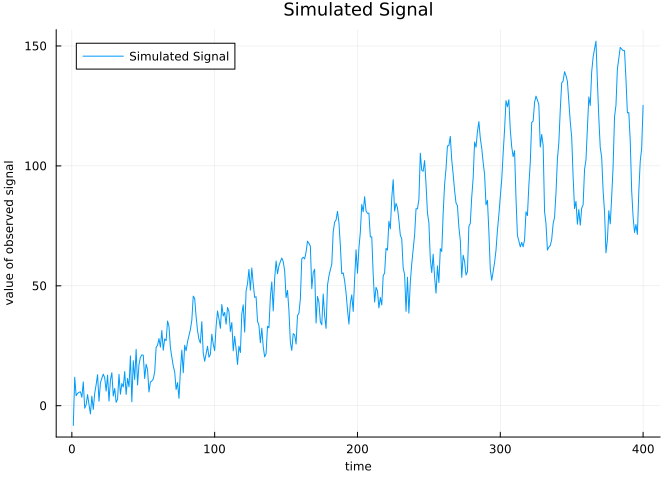
To better understand we will work through recovering the components of a toy series. The length of this series is taken as $N = 400$ points, described as

$$x(i)=0.3i+(1+0.1i)\sin\left(\frac{2\pi}{20}i\right)$$

The signal is then pertubated with gaussian noise, which is calculated with the following function.

function gaussian_noise(sigma,signal)
    signal_dim=length(signal)
    noise = sigma .* randn(signal_dim)
    return noise
end

Taking the sigma=5. This gives us our observed signal that we will work with.

Embedding

The embedding step is governed by the choice of the parameter, L. The basic idea behind choosing L is to capture the structure that underlies the signal within each lagged vector.

If the length is too small, then the pattern can be split between different lags. While this can be useful is extracting localized features for most cases we want to over compensate by taking a larger window. While this affects our computational time, we will focus on optimizing other steps to accomodate.

The usual rule, is to chose $L$, close to the half the length of the signal.

$$L\leq \frac{N}{2}$$

In our example we will choose this to be about 180. Then using our formula for K, we have

$$K = N - L + 1 = 400-180+1 = 221$$

Using these calculated value we can intialize the matrix with the dimensions $K \times L = 221\times 180$.

Then using Equation 1, which is $X_{i,j} = x_{i+j-1}$, we can make a function that loops through L and K, and assigns the values to the Trajectory matrix.

We can make a function for this

function trajectory_matrix = hankel(x,L)
  N = length(x);
  K = N - L + 1;

  X = zeros(K, L);

  for i = 1:K
    for j = 1:L
      X(i,j) = x(i + j - 1);
    endfor
  endfor

  trajectory_matrix = X;
endfunction

SVD or Partial SVD

Implimenting SVD is rather easy for almost any scientific computing language. Most have functions built into them, like Octave, or have well supported libraries like LinearAlgebra.jl in Julia.

The only change I have made in my implementation within Octave is to pass the singular values as a vector instead of a Diagonal Matrix.

function [U, S, V] = svd_vals(X)
  [U, S_diagonal, V] = svd(X);

  S = diag(S_diagonal);
endfunction

Now in terms of efficiency this is one of the points at which we can often hit a brick in computation time when calculating the full SVD of a matrix. One of the time-series we will do our application on is about 760000 data points. Choosing $L=32000$ we are taking the SVD of a $44000 \times 32000$. The task takes far too long.

The optimization at this step are suggested within Lopes et al. (2024), the two suggestions mainly are Partial SVDs and Randomized SVDs.

Partial SVD is built in within Octave, where we can simply calculate a chosen, $k$, number of eigentriples and get them

function [U, S, V] = optim_svd(X, k)
  [U, S_diagonal, V] = svds(X, k);

  S = diag(S_diagonal);
endfunction

While faster than normal SVD, this step still can be very taxing. The alternative is Random SVD. Here it uses a probabilistic method to find chosen, $k$ eigentriples of the original matrix. This method when implimented was used using the LowRankApprox.jl package within julia as there aren’t any packages built within Octave.

Now after obtaining the decompositon $U, \Sigma, V$, we then usually move onto the grouping stage. But to allow for better efficiency it is often better to develop the reconstructed matrices for chosen $k$ eigentriples.

So we will now first develop the Diagonal Averaging algorithm and get our reconstructed series, which for rank-1 matrices we will refer to as elementary reconstructions.

Diagonal Averaging (Hankelization to obtain time series)

As we discussed our theory behind converting these rank-1 matrices into Hankelized version of themselves and then extracting the time series by simply taking the values of each anti-diagonal.

Hankelization works simply by summing the values of each anti-diagonal and dividing by the number of terms in that anti-diagonal. We will first code an algorithm that makes a vector of the counts of terms in each diagonal. This function is separated as this vector is also useful during our grouping stage as it is also the weights used in W-correlation matrix.

The weights are defined as

$$w_n = \begin{cases} n, & 1 \le n \le L \\[6pt] L, & L \le n \le K \\[6pt] N - n + 1, & K \le n \le N \end{cases}$$

given that $N=K+L-1$

this can simply be coded as

function weight = weights(L, K)
  N = K + L - 1;
  weight = zeros(1, N);

  for n = 1:N
    weight(n) = min([n, L, N - n + 1]);
  end
end

Now we simply have to calculate another vector which sums the values of each anti-diagonal, and divide the two vectors element-wise to obtain our reconstructed series. Now, as terms on each anti-diagonal have equal sums of their indices, we can program a looping algorithm that goes through each element of the matrix and simply adds the values of current term to its corresponsing index in our anti-diagonal sum series.

Now as this function works mainly to evaluate elementary reconstructed series, we pass decomposed $u_i,\sigma_i,v_i$ to this function. Instead of also evaluating the whole matrix and using memory for that, we just evaluate each term of the matrix.

function series = hankelized_series(u, sigma, v)
  K = length(u);
  L = length(v);
  N = K + L - 1;

  a_diag_sum = zeros(1, N);
  counts = weights(L, K);

  for j = 1:L
    v_j = v(j);

    for i = 1:K
      n = i + j - 1;
      a_diag_sum(n) = a_diag_sum(n) + sigma * u(i) * v_j;
    end
  end

  series = a_diag_sum ./ counts;
end

We can then code a function to store the first, $k$ elementary reconstructed series. They are stored in a cell within Octave but can be stored as just vectors inside a vector in Julia.

function elementary_recons = elementary_reconstructions(U, Sigma, V, k)
  K = size(U, 1);
  L = size(V, 1);

  N = K + L - 1;

  elementary_recons = cell(1, k);

  for i = 1:k
    elementary_recons{i} = hankelized_series(U(:, i), Sigma(i), V(:, i));
  end
end

The choice of k, here is rather arbitary. One of the ways we can make this choice, or atleast consider the minimum for it, is by analyzing a crucial graph within SSA, the graph of the singular values. This transitions us into the final step, Grouping.

Grouping

This stage is the most involved in terms of human input. Which also gives us the opportunity to impliment more automatic methods and better understand SSA.

First assuming we have our groups, we need a way to sum the elementary reconstructions corresponding to the terms in each group. This can be done by the following function

function grouped_recons = grouped_series(elementary_recons, L, K, groups)

  n = length(groups);
  N = K + L - 1;

  grouped_recons = cell(1, n);

  for i = 1:n
    grouped_recons{i} = zeros(1, N);

    for j = groups{i}
      grouped_recons{i} = grouped_recons{i} + elementary_recons{j};
    end
  end

end

Singular Values : SSA for Signal + Noise model

We often first begin by simply plotting the singular values, we obtained during our SVD step. Plotting this for our Simulated Toy series :

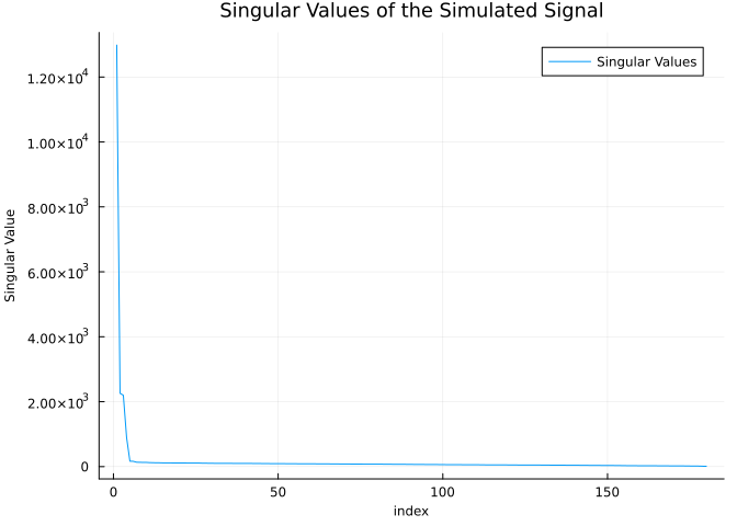
It is important to note that the nature of the plot. It confirms our earlier discussion that the main structure of the series is associated with the highest singular values, and then as noise is spread in many directions, each component of it contributes very little.

This kind of plot is a scree plot. We can It serves as the first way for us to identify a basic grouping, especially for the model $S_{observed} = S_{signal} + N$, where $N$ is the noise. The point at which the graph starts to flatten seems a natural place to split our Signal and Noise. This is often reffered to as the elbow point.

We can also make this plot easier to understand by taking the log, and scaling this and also labeling the point at which signal drops off.

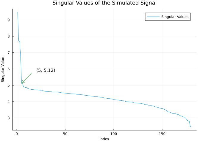
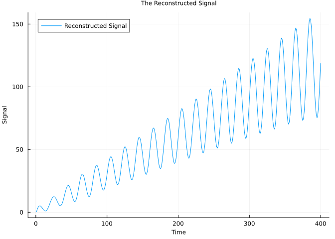
Then we have our groups for Signal being $1:5$ and the residual/noise being $3:\text{length(S)}$. Plotting our reconstructed signal and the observed signal we have :

We can also compare the reconstructed signal to our true signal,

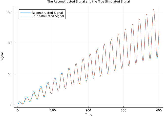
We can quantify the quality of this smoothing by calculating the Root Mean Squared Error. Its the error relative to our signal.

$$\mathrm{RMSE} = \sqrt{\mathbb{E}\left[(X - \hat{X})^2\right]}$$

This measures the average deviation of our reconstruction compared to the original function.

For our reconstructed signal compared to original, it is $1.621$, comparing this to the range of the original signal, our Relative error is about $0.01$. We will use this measure as our relative error in this paper.

The residual can also be plotted,

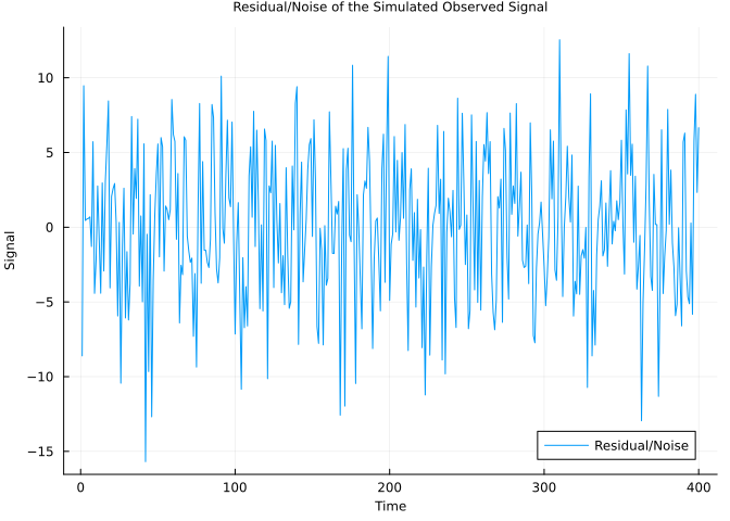
This covers our work on implimenting SSA for the naive signal model. It simply becomes the task of approximating the elbow of our singular value scree plot.

Grouping for Trend and Periodic components

The goal of grouping is also to recover the underlying seperable components. As we discussed earlier this can be done by finding groups where their W-correlation is close to 1, as these elementary reconstruction series would be closer to each other and hence should be part of the same groups.

We can do this by creating our W-correlation matrix and then creating a heatmap of this matrix.

We can calculate this matrix and create an heatmap within octave with the following function, passing it the elementary reconstructions and the number of reconstructions for which we are interested in creating the heatmap for, $k$.

function rho = w_heatmap(elementary_recons, L, K, k)
  weight = weights(L, K);
  N = L + K - 1;

  recon_matrix = zeros(k, N);
  weighted_matrix = zeros(k, N);

  for i = 1:k
    recon_matrix(i, :) = elementary_recons{i};
    weighted_matrix(i, :) = elementary_recons{i} .* weight;
  end

  W = recon_matrix * weighted_matrix';

  norms = sqrt(diag(W));
  rho = W ./ (norms * norms');

  rho = abs(rho);

  figure;
  imagesc(rho);
  colormap(gray);
  colorbar;
  caxis([0 1]);
  xlabel('i');
  ylabel('j');
  title('Grayscale Heatmap');

end

Producing this heatmap for the first 15 eigentriples we get.

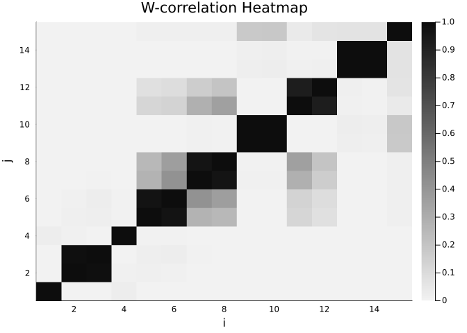
Focusing on all groupings that exist until only the 6 eigentriple, as this is where our signal can best be reconstructed from, we have the following groups : [1,2:3,4,5:6]. These are the components that were highly correlated with each other, a W-correlation score close to 1.

These can be interpreted in the following manner. The easiest is to simply graph these groups as that would make it much more obvious as to which ones are trend and ones with oscillation.

An important property of components associated with oscillatory components is that they typically appear in pairs. This arises from the fact that any oscillation can be represented as a linear combination of sine and cosine functions of the same frequency. These two functions form an orthogonal basis for a two-dimensional subspace capturing that oscillatory pattern. Since SVD identifies orthogonal spaces, it naturally extracts two components spanning this subspace. As a result, oscillatory modes are represented by pairs of components that are often highly correlated.

This also gives rise to an elegant graph where when the right singular vector associated with one in the pair is graphed against the other we get a structure approximating a circle.

We generate these plot for the two pairs that appear in our grouping.

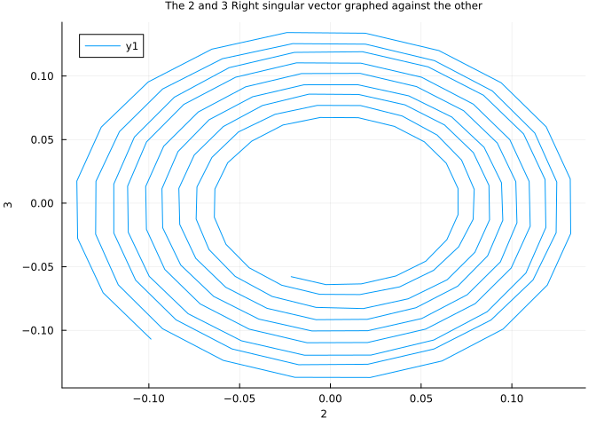
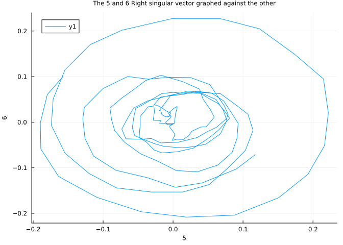
We can then plot the reconstructed component series of each group to understand its nature better.

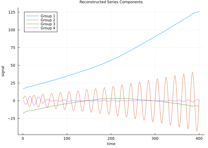
This confirms our discussion earlier, that those groups that exist as a pair. The other two groups, which have a single term seem to be the overall trend. This now allows us to some these components and extract the signals appropriate trend and oscillation.

We can do this by passing another grouping to our reconstructed series function and get graph these.

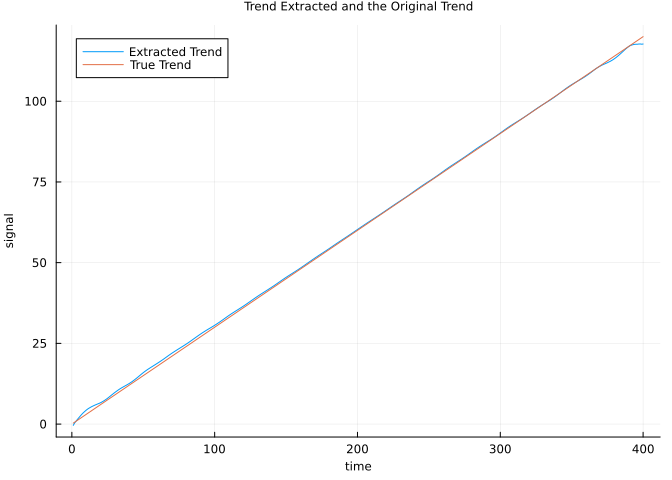
Our relative error between the extracted trend and original trend is 0.5%.

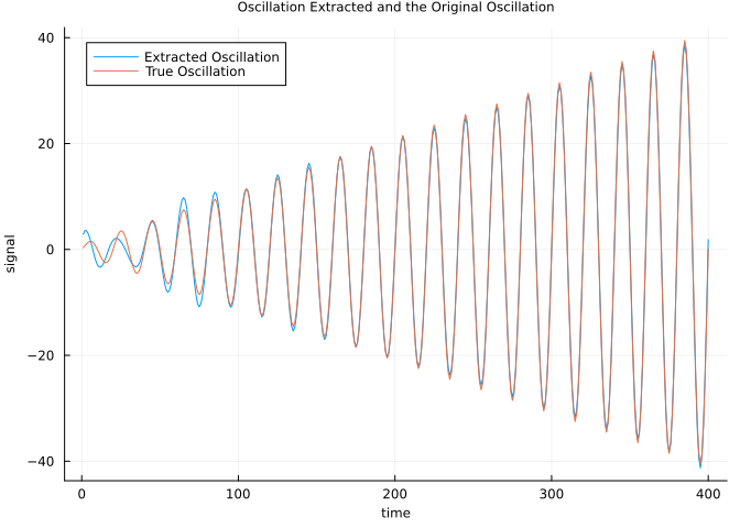
Our relative error between the extracted oscillation and original oscillation is 0.9%.

This covers our basic implementation for an SSA algorithm where we find a smoothing of the observed signal and also extract its components.

The implementation of this example is followed in the file toy_signal.m

Example Applications of SSA

Light Curve of a White Dwarf

The following time series analyzed in this section consists of observations of the light curve of the variable white dwarf star PG1159-035. The data was recorded in March 1989 using the Whole Earth Telescope, a coordinated network of telescopes designed to enable continuous astronomical observations.

The measurements represent the variation in observed light intensity over time and were sampled at regular intervals of 10 seconds. This dataset contains 618 observations from a single continuous interval.

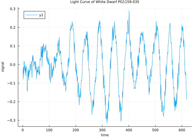
Given $N=618$ we can choose an $L=280$, and create our Trajectory matrix and take its SVD. Graphing the singular values we have, the following scree plot :

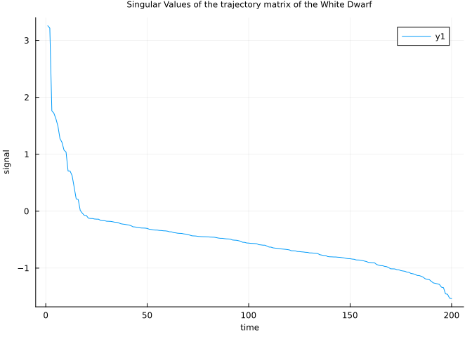
From this graph, we can see that the elbow is at $k=11$, after which the plot falls off and starts to flatten suggesting only contribution from noise. This allows us to create our initial groupings for a $S_{observed}=S_signal+N$ model.

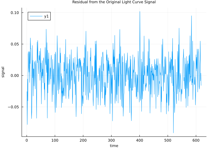
To extract any components we can analyze the W-Correlation Heatmap.

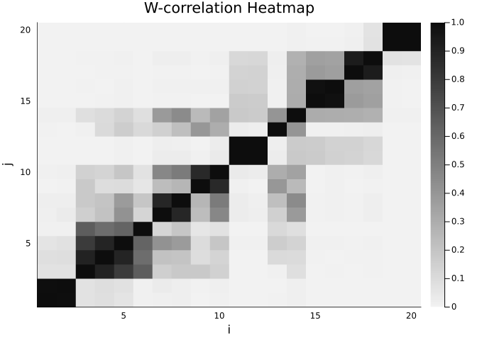
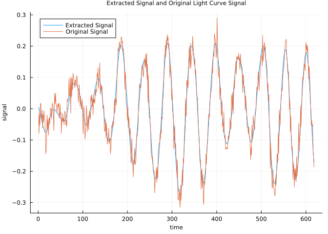
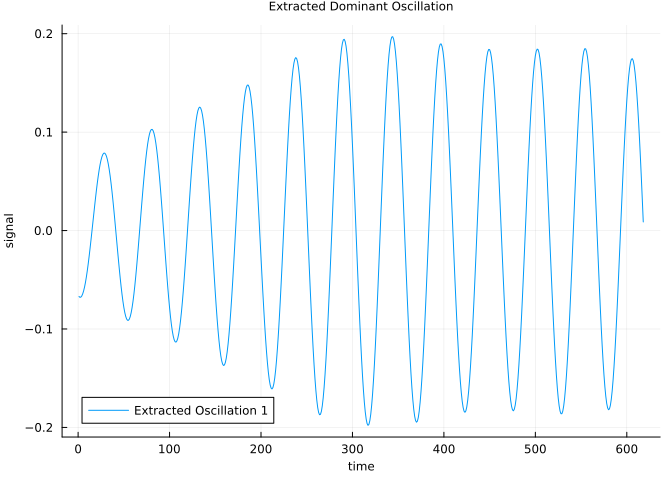
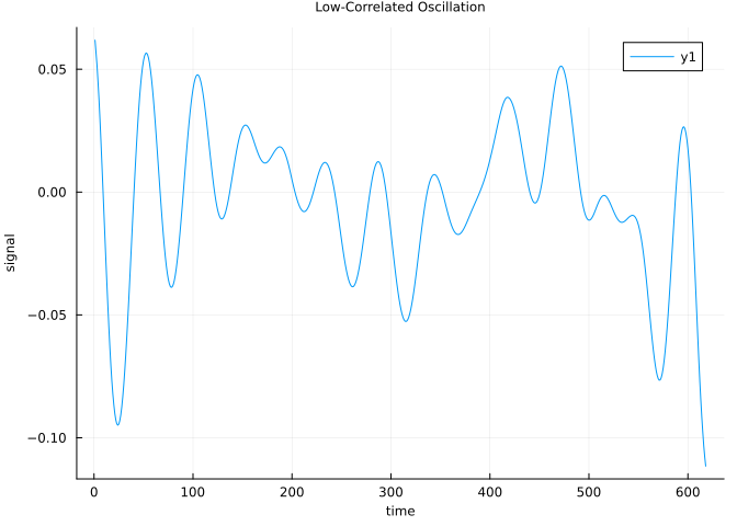
Here the main extractable component is the first group pair (1,2) which is the dominating oscillation. There are also some-what correlated pairs (3,4,5) Which seem to two other oscillations that bleed into each other.

Graphing these reconstruction we get the following extracted oscillation.

Daily sunspots data

The following is the number of Daily sunspot number collected since 1/1/1818 till now as shared in Clette et al. (2015). Our goal will be to extract the oscillatory or seasonal component from this dataset to evaluate for ourselves the period of the Sunspot Cycle.

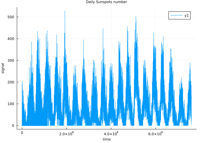
There are approximately 76000 datapoints. Taking $L=32000$, We are working with a trajectory matrix of approximately $32000\times44000$ dimensions. This allows us to implement a Randomized SVD for performing SSA. As both full SVD and partial SVD taking far too long for such dense matrix.

Choosing the first $k=20$ eigentriples to focus on, plotting the singular values we have :

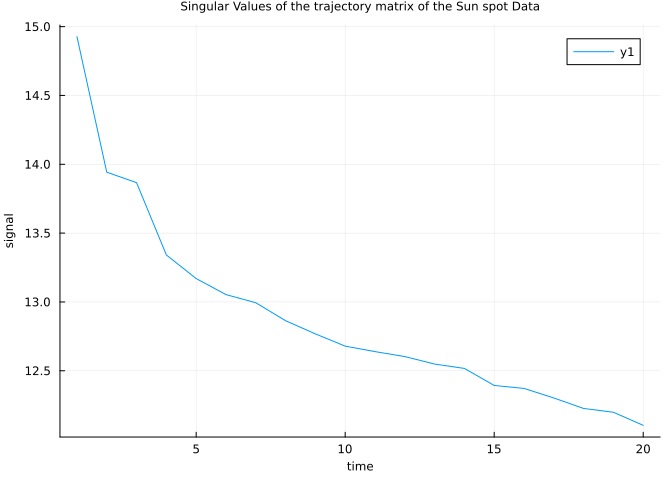
We can see that the majority of the observed data has a structure contributing ot it until the 3 eigentriple.

We can further analyze the W-Correlation Heatmap as well.

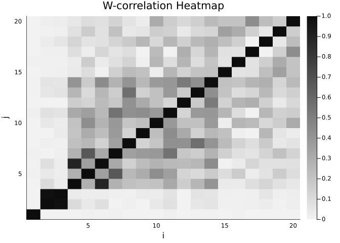
This suggests the two groups : 1 and (2,3). Graphing the two extracted components :

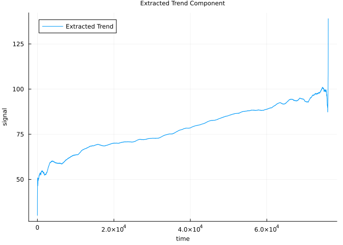
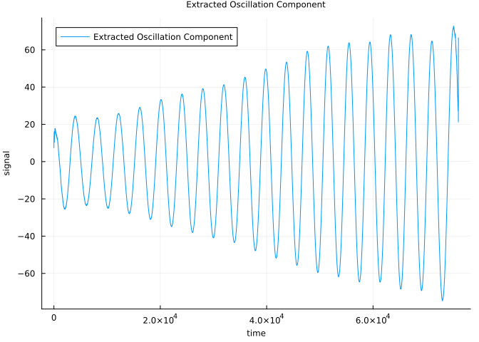
We can now simply even calculate the period from the Oscillatory component as the other major one is simply the trend. Our extraction suggests a period of approximately 10.9 years. The accepted period for Sunspot periods by NASA is 11 years. This confirms our extraction from a noisy data where about 15% of the data is missing, is still very accurate.

Conclusion

Singular Spectrum Analysis (SSA) provides a powerful and flexible way to decompose a time series without assuming a fixed basis in advance. It is adaptive in its approac. By embedding the original series into a trajectory matrix and applying SVD, we are able to re-express our matrix by highlighting the main structures first. This allows dominant patterns, oscillations, trends, and noise to be separated through the singular values, reconstructed components, and W-correlation matrix.

Through the simulated example, SSA has been shown to recover both the trend and oscillatory components with low relative error. The white dwarf light curve example demonstrated how SSA can extract meaningful oscillatory behavior from real astrophysical data, while the sunspot example showed that SSA can recover the well-known approximately 11-year solar cycle from noisy, incomplete observations.

Overall, SSA is useful because it combines interpretability with adaptability. Its effectiveness depends strongly on appropriate choices of window length, rank truncation, and grouping, but its fast implimentation allows one to play around with these parameters until a viable result can be reached. This confirms SSA as a practical method for smoothing, denoising, and extracting meaningful structure from complex time series.

References

1. Clette, F., Svalgaard, L., Vaquero, J. M., & Cliver, E. W. (2015). Revisiting the Sunspot Number: A 400-year perspective on the solar cycle. Space Science Reviews, 186(1-4), 35-103.
2. Elsner, J. B., & Tsonis, A. A. (1996). Singular Spectrum Analysis: A New Tool in Time Series Analysis. Springer.
3. Golyandina, N., Nekrutkin, V., & Zhigljavsky, A. (2001). Analysis of Time Series Structure: SSA and Related Techniques. Chapman & Hall/CRC.
4. Golyandina, N., & Zhigljavsky, A. (2020). Particularities and commonalities of singular spectrum analysis as a method of time series analysis and signal processing. WIREs Computational Statistics, 12(4), e1487.
5. Lopes, F., Gibert, D., Courtillot, V., Le Mouël, J.-L., & Boulé, J.-B. (2024). On the optimization of singular spectrum analyses: A pragmatic approach. arXiv preprint arXiv:2412.17793.